
[1]:
%run notebook_setup
If you have not already read it, you may want to start with the first tutorial: Getting started with The Joker.
Sampling over long-term velocity trend parameters#
In addition to the default linear parameters (see Tutorial 1, or the documentation for JokerSamples.default()), The Joker allows adding linear parameters to include a long-term polynomial velocity trend. While The Joker formally only works for the two-body problem, if the system is a triple, and the outer body is in a significantly longer period orbit, you may be able to represent its perturbation to the primary as a smooth polynomial (in time) over the
observation window you have. Below, we will show this with an example
First, some imports we will need later:
[2]:
import astropy.table as at
import astropy.units as u
import numpy as np
import thejoker as tj

%matplotlib inline
WARNING (pytensor.tensor.blas): Using NumPy C-API based implementation for BLAS functions.
[3]:
# set up a random number generator to ensure reproducibility
rnd = np.random.default_rng(seed=123)
Let’s start by loading some pre-generated data meant to represent radial velocity observations of a single luminous source with two faint companions: one on a shorter period orbit, the other with a period ~ 10x longer.
[4]:
data = tj.RVData.guess_from_table(at.QTable.read("data-triple.ecsv"))
data = data[rnd.choice(len(data), size=16, replace=False)]  # downsample data
[5]:
_ = data.plot()
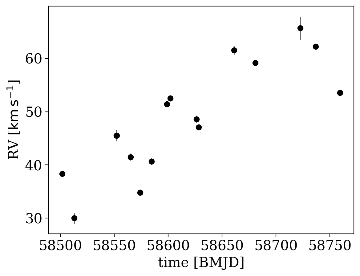
Let’s first pretend that we don’t know it is a triple, and try generating orbit samples assuming a binary with no polynomial velocity trend. We will set up the default prior with some reasonable parameters that we have used in previous tutorials, and generate a big cache of prior samples:
[6]:
prior = tj.JokerPrior.default(
    P_min=2 * u.day,
    P_max=1e3 * u.day,
    sigma_K0=30 * u.km / u.s,
    sigma_v=100 * u.km / u.s,
)
prior_samples = prior.sample(size=250_000, rng=rnd)
Now we can run The Joker to generate posterior samples:
[7]:
joker = tj.TheJoker(prior, rng=rnd)
samples = joker.rejection_sample(data, prior_samples, max_posterior_samples=128)
samples
[7]:
<JokerSamples [P, e, omega, M0, s, K, v0] (1 samples)>
[8]:
_ = tj.plot_rv_curves(samples, data=data)
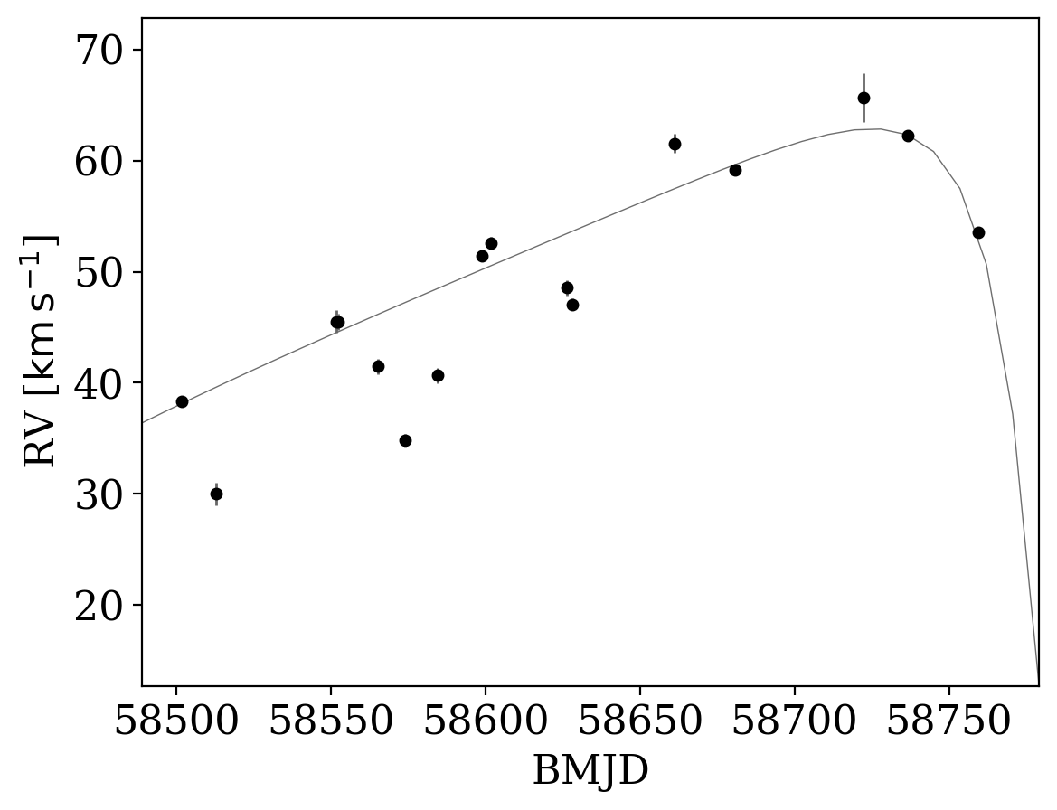
Only one sample was returned, and it’s not a very good fit to the data (see the plot above). This is because the data were generated from a hierarchical triple system, but fit as a two-body system. Let’s now try generating Keplerian orbit samples for the inner binary, while including a polynomial trend in velocity to capture the long-term trend from the outer companion. To do this, we specify the number of polynomial trend coefficients to sample over: 1 is constant, 2 is linear, 3 is quadratic, etc. We also have to specify the standard deviations of the Gaussian priors on the trend parameters, so the units have to be set accordingly:
[9]:
prior_trend = tj.JokerPrior.default(
    P_min=2 * u.day,
    P_max=1e3 * u.day,
    sigma_K0=30 * u.km / u.s,
    sigma_v=[100 * u.km / u.s, 0.5 * u.km / u.s / u.day, 1e-2 * u.km / u.s / u.day**2],
    poly_trend=3,
)
Notice the additional parameters v1, v2 in the prior:
[10]:
prior_trend
[10]:
<JokerPrior [P, e, omega, M0, s, K, v0, v1, v2]>
We are now set up to generate prior samples and run The Joker including the new linear trend parameters:
[11]:
prior_samples_trend = prior_trend.sample(size=250_000, rng=rnd)
joker_trend = tj.TheJoker(prior_trend, rng=rnd)
samples_trend = joker_trend.rejection_sample(
    data, prior_samples_trend, max_posterior_samples=128
)
samples_trend
[11]:
<JokerSamples [P, e, omega, M0, s, K, v0, v1, v2] (1 samples)>
[12]:
_ = tj.plot_rv_curves(samples_trend, data=data)
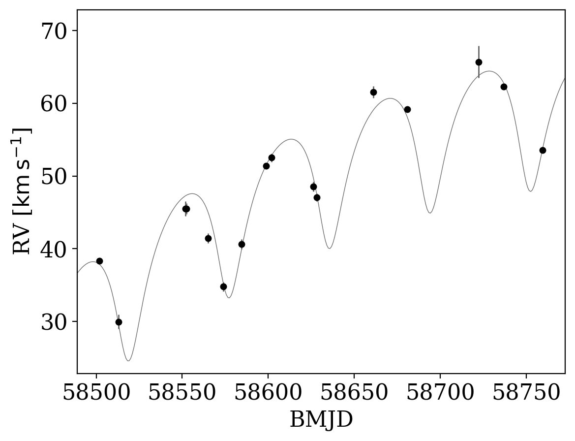
Those orbit samples look much better at matching the data! In a real-world situation with these data and results, given that the samples look like they all share a similar period, at this point I would start standard MCMC to continue generating samples. But, that is covered in Tutorial 4, so for now, we will proceed with only the samples returned from The Joker.
So how do the sample values compare to the truth? I cached the true orbital parameter values for the inner binary of this system:
[13]:
import pickle

with open("true-orbit-triple.pkl", "rb") as f:
    truth = pickle.load(f)
Truth:
[14]:
truth["P"], truth["e"], truth["K"]
[14]:
(<Quantity 58.63210685 d>, <Quantity 0.25>, <Quantity 7.37900547 km / s>)
Assuming binary:
[15]:
samples["P"], samples["e"], samples["K"]
[15]:
(<Quantity [546.13967944] d>,
 <Quantity [0.674905]>,
 <Quantity [-51.76894619] km / s>)
Assuming binary + quadratic velocity trend:
[16]:
samples_trend.mean()["P"], samples_trend.mean()["e"], samples_trend.mean()["K"]
[16]:
(<Quantity [58.39243129] d>,
 <Quantity [0.31584264]>,
 <Quantity [8.79219835] km / s>)
The period and semi-amplitude values we infer from including the velocity trend is less biased. Hurrah!