
[1]:
%run notebook_setup
If you have not already read it, you may want to start with the first tutorial:Getting started with The Joker.
Continue generating samples with standard MCMC#
When many prior samples are used with The Joker, and the sampler returns one sample, or the samples returned are within the same mode of the posterior, the posterior pdf is likely unimodal. In these cases, we can use standard MCMC methods to generate posterior samples, which will typically be much more efficient than The Joker itself. In this example, we will use pymc3 to “continue” sampling for data that are very constraining.
First, some imports we will need later:
[2]:
import astropy.coordinates as coord
import astropy.table as at
import astropy.units as u
import numpy as np
import corner
import pymc as pm
import arviz as az
import thejoker as tj

%matplotlib inline
WARNING (pytensor.tensor.blas): Using NumPy C-API based implementation for BLAS functions.
[3]:
# set up a random number generator to ensure reproducibility
rnd = np.random.default_rng(seed=8675309)
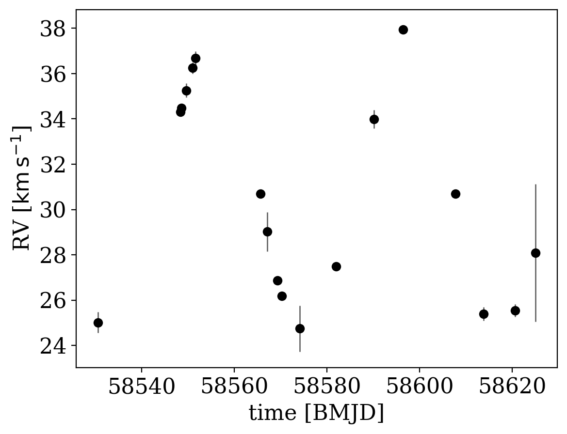
Here we will again load some pre-generated data meant to represent well-sampled, precise radial velocity observations of a single luminous source with a single companion (we again downsample the data set here just for demonstration):
[4]:
data_tbl = at.QTable.read("data.ecsv")
sub_tbl = data_tbl[rnd.choice(len(data_tbl), size=18, replace=False)]  # downsample data
data = tj.RVData.guess_from_table(sub_tbl, t_ref=data_tbl.meta["t_ref"])
[5]:
_ = data.plot()
We will use the default prior, but feel free to play around with these values:
[6]:
prior = tj.JokerPrior.default(
    P_min=2 * u.day,
    P_max=1e3 * u.day,
    sigma_K0=30 * u.km / u.s,
    sigma_v=100 * u.km / u.s,
)
The data above look fairly constraining: it would be hard to draw many distinct orbital solutions through the RV data plotted above. In cases like this, we will often only get back 1 or a few samples from The Joker even if we use a huge number of prior samples. Since we are only going to use the samples from The Joker to initialize standard MCMC, we will only use a moderate number of prior samples:
[7]:
prior_samples = prior.sample(size=250_000, rng=rnd)
[8]:
joker = tj.TheJoker(prior, rng=rnd)
joker_samples = joker.rejection_sample(data, prior_samples, max_posterior_samples=256)
joker_samples
[8]:
<JokerSamples [P, e, omega, M0, s, K, v0] (1 samples)>
[9]:
joker_samples.tbl
[9]:
| P | e | omega | M0 | s | K | v0 |
|---|---|---|---|---|---|---|
| d | rad | rad | km / s | km / s | km / s | |
| float64 | float64 | float64 | float64 | float64 | float64 | float64 |
| 42.124700811110955 | 0.07897171939998879 | 1.2128740697412264 | 1.4532453531640455 | 0.0 | 6.70834451543562 | 31.171646942585795 |
[10]:
_ = tj.plot_rv_curves(joker_samples, data=data)
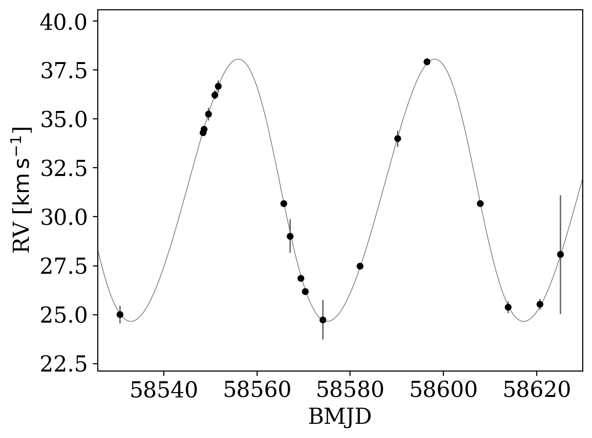
The sample that was returned by The Joker does look like it is a reasonable fit to the RV data, but to fully explore the posterior pdf we will use standard MCMC through pymc3. Here we will use the NUTS sampler, but you could also experiment with other backends (e.g., Metropolis-Hastings, or even emcee by following this blog post):
[11]:
with prior.model:
    mcmc_init = joker.setup_mcmc(data, joker_samples)

    trace = pm.sample(tune=500, draws=500, start=mcmc_init, cores=1, chains=2)
Auto-assigning NUTS sampler...
Initializing NUTS using jitter+adapt_diag...
Sequential sampling (2 chains in 1 job)
NUTS: [e, __omega_angle1, __omega_angle2, __M0_angle1, __M0_angle2, P, K, v0]
/opt/hostedtoolcache/Python/3.11.9/x64/lib/python3.11/site-packages/rich/live.py:231: UserWarning: install
"ipywidgets" for Jupyter support
  warnings.warn('install "ipywidgets" for Jupyter support')
Sampling 2 chains for 500 tune and 500 draw iterations (1_000 + 1_000 draws total) took 30 seconds.
We recommend running at least 4 chains for robust computation of convergence diagnostics
If you get warnings from running the sampler above, they usually indicate that we should run the sampler for many more steps to tune the sampler and for our main run, but let’s ignore that for now. With the MCMC traces in hand, we can summarize the properties of the chains using pymc3.summary:
[12]:
az.summary(trace, var_names=prior.par_names)
/opt/hostedtoolcache/Python/3.11.9/x64/lib/python3.11/site-packages/arviz/stats/diagnostics.py:596: RuntimeWarning: invalid value encountered in scalar divide
  (between_chain_variance / within_chain_variance + num_samples - 1) / (num_samples)
[12]:
| mean | sd | hdi_3% | hdi_97% | mcse_mean | mcse_sd | ess_bulk | ess_tail | r_hat | |
|---|---|---|---|---|---|---|---|---|---|
| P | 42.135 | 0.137 | 41.904 | 42.407 | 0.006 | 0.004 | 563.0 | 498.0 | 1.01 |
| e | 0.097 | 0.015 | 0.070 | 0.125 | 0.001 | 0.000 | 437.0 | 483.0 | 1.00 |
| omega | 1.165 | 0.120 | 0.954 | 1.410 | 0.006 | 0.004 | 413.0 | 485.0 | 1.01 |
| M0 | 1.393 | 0.127 | 1.162 | 1.646 | 0.007 | 0.005 | 374.0 | 484.0 | 1.01 |
| s | 0.000 | 0.000 | 0.000 | 0.000 | 0.000 | 0.000 | 1000.0 | 1000.0 | NaN |
| K | 6.745 | 0.098 | 6.557 | 6.919 | 0.004 | 0.003 | 721.0 | 840.0 | 1.00 |
| v0 | 31.199 | 0.061 | 31.080 | 31.310 | 0.003 | 0.002 | 537.0 | 645.0 | 1.00 |
To convert the trace into a JokerSamples instance, we can use the TheJoker.trace_to_samples() method. Note here that the sign of K is arbitrary, so to compare to the true value, we also call wrap_K() to store only the absolute value of K (which also increases omega by π, to stay consistent):
[13]:
mcmc_samples = tj.JokerSamples.from_inference_data(prior, trace, data)
mcmc_samples.wrap_K()
mcmc_samples
[13]:
<JokerSamples [P, e, omega, M0, s, K, v0, ln_posterior, ln_likelihood, ln_prior] (1000 samples)>
We can now compare the samples we got from MCMC to the true orbital parameters used to generate this data:
[14]:
import pickle

with open("true-orbit.pkl", "rb") as f:
    truth = pickle.load(f)

# make sure the angles are wrapped the same way
if np.median(mcmc_samples["omega"]) < 0:
    truth["omega"] = coord.Angle(truth["omega"]).wrap_at(np.pi * u.radian)

if np.median(mcmc_samples["M0"]) < 0:
    truth["M0"] = coord.Angle(truth["M0"]).wrap_at(np.pi * u.radian)
[15]:
df = mcmc_samples.tbl.to_pandas()
truths = []
colnames = []
for name in df.columns:
    if name in truth:
        colnames.append(name)
        truths.append(truth[name].value)
_ = corner.corner(df[colnames], truths=truths)
WARNING:root:Pandas support in corner is deprecated; use ArviZ directly
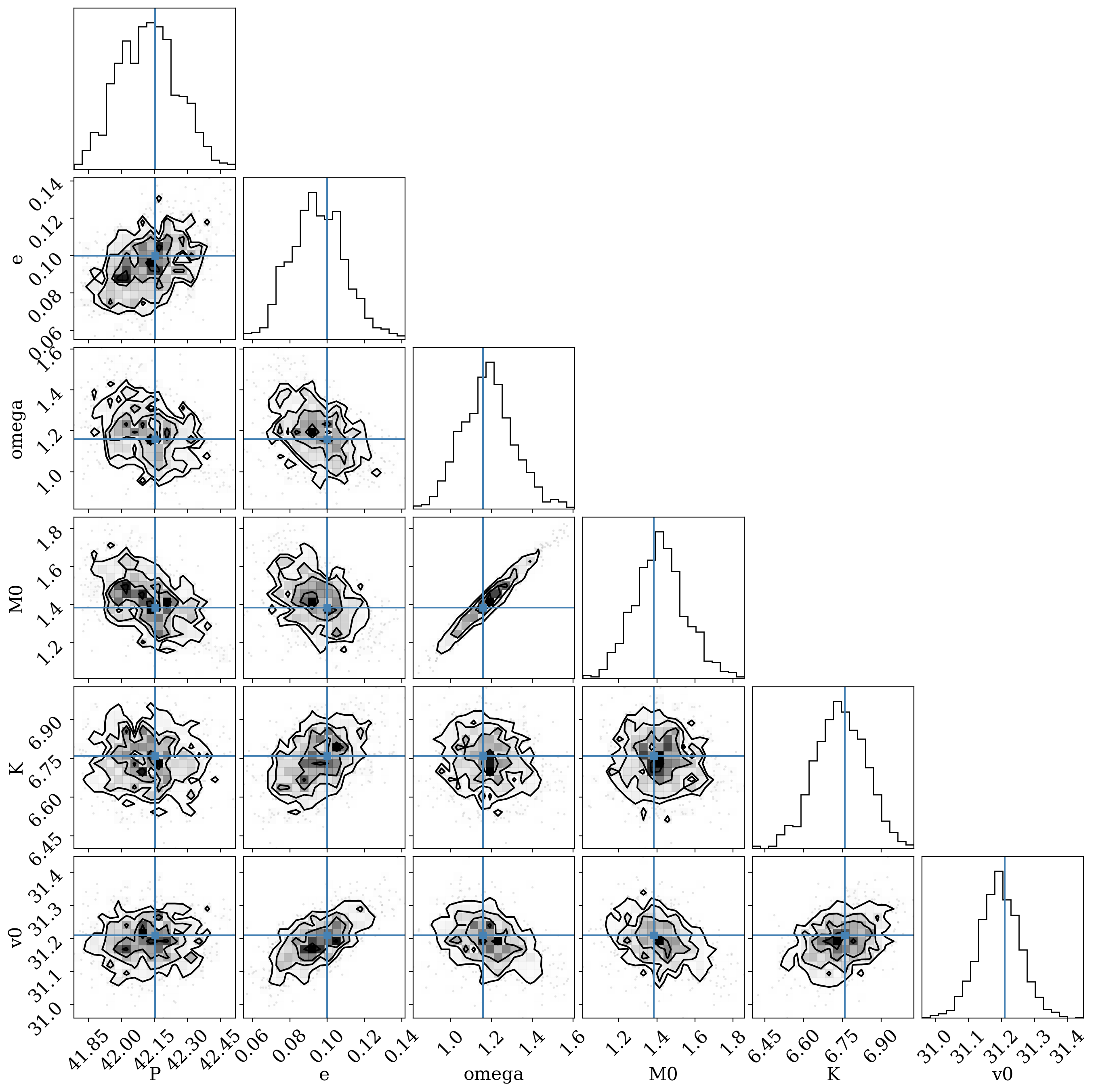
Overall, it looks like we do recover the input parameters!