
[1]:
%run notebook_setup
Reproducing the black hole discovery in Thompson et al. 2019#
In this science demo tutorial, we will reproduce the results in Thompson et al. 2019, who found and followed-up a candidate stellar-mass black hole companion to a giant star in the Milky Way. We will first use The Joker to constrain the orbit of the system using the TRES follow-up radial velocity data released in their paper and show that we get consistent period and companion mass constraints from modeling these data. We will then do a joint analysis of the TRES and APOGEE data for this source by simultaneously fitting for and marginalizing over an unknown constant velocity offset between the two surveys.
A bunch of imports we will need later:
[2]:
import arviz as az
import astropy.units as u
import corner
import matplotlib.pyplot as plt
import numpy as np
import pymc as pm
import thejoker as tj
import thejoker.units as xu
from astropy.io import ascii
from astropy.time import Time

%matplotlib inline
WARNING (pytensor.tensor.blas): Using NumPy C-API based implementation for BLAS functions.
[3]:
# set up a random number generator to ensure reproducibility
seed = 42
rnd = np.random.default_rng(seed=seed)
Load the data#
We will start by loading data, copy-pasted from Table S2 in Thompson et al. 2019):
[4]:
tres_tbl = ascii.read(
    """8006.97517 0.000 0.075
    8023.98151 -43.313 0.075
    8039.89955 -27.963 0.045
    8051.98423 10.928 0.118
    8070.99556 43.782 0.075
    8099.80651 -30.033 0.054
    8106.91698 -42.872 0.135
    8112.81800 -44.863 0.088
    8123.79627 -25.810 0.115
    8136.59960 15.691 0.146
    8143.78352 34.281 0.087""",
    names=["HJD", "rv", "rv_err"],
)
tres_tbl["rv"].unit = u.km / u.s
tres_tbl["rv_err"].unit = u.km / u.s
[5]:
apogee_tbl = ascii.read(
    """6204.95544 -37.417 0.011
    6229.92499 34.846 0.010
    6233.87715 42.567 0.010""",
    names=["HJD", "rv", "rv_err"],
)
apogee_tbl["rv"].unit = u.km / u.s
apogee_tbl["rv_err"].unit = u.km / u.s
[6]:
tres_data = tj.RVData(
    t=Time(tres_tbl["HJD"] + 2450000, format="jd", scale="tcb"),
    rv=u.Quantity(tres_tbl["rv"]),
    rv_err=u.Quantity(tres_tbl["rv_err"]),
)

apogee_data = tj.RVData(
    t=Time(apogee_tbl["HJD"] + 2450000, format="jd", scale="tcb"),
    rv=u.Quantity(apogee_tbl["rv"]),
    rv_err=u.Quantity(apogee_tbl["rv_err"]),
)
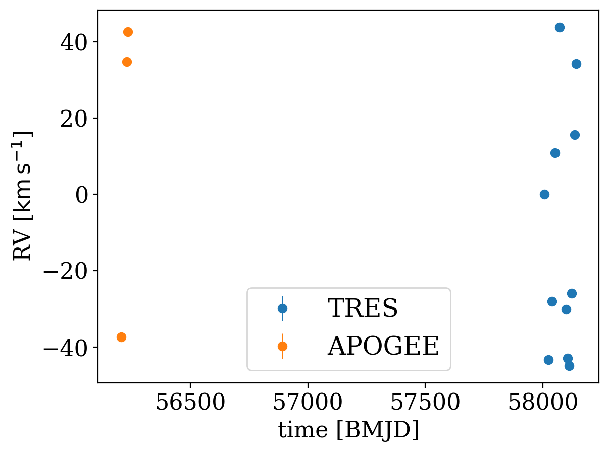
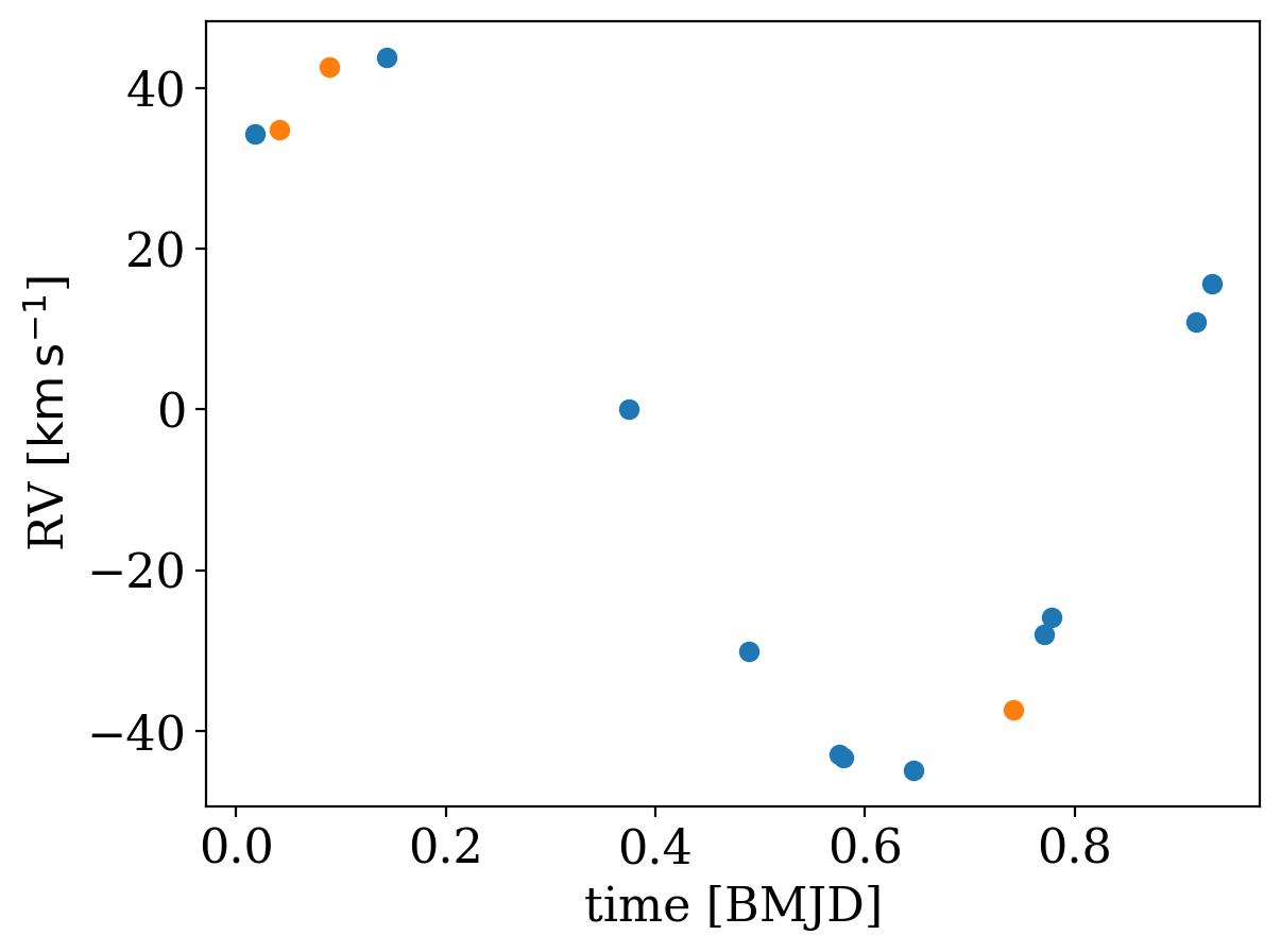
Let’s now plot the data from these two instruments:
[7]:
for d, name in zip([tres_data, apogee_data], ["TRES", "APOGEE"]):
    d.plot(color=None, label=name)
plt.legend(fontsize=18)
[7]:
<matplotlib.legend.Legend at 0x7fa38f23de10>
Run The Joker with just the TRES data#
The two data sets are separated by a large gap in observations between the end of APOGEE and the start of the RV follow-up with TRES. Since there are more observations with TRES, we will start by running The Joker with just data from TRES before using all of the data. Let’s plot the TRES data alone:
[8]:
_ = tres_data.plot()
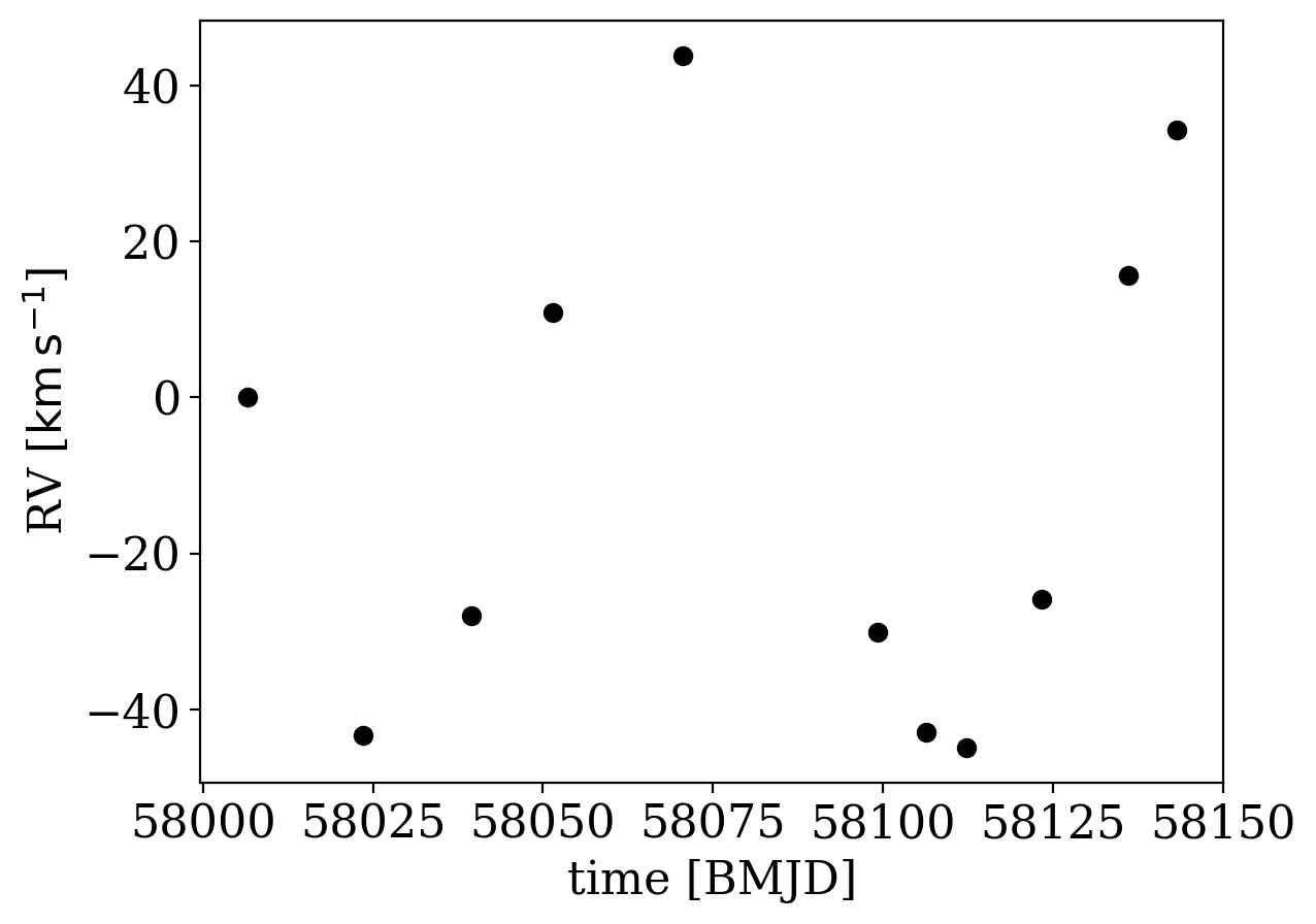
It is pretty clear that there is a periodic signal in the data, with a period between 10s to ~100 days (from eyeballing the plot above), so this limits the range of periods we need to sample over with The Joker below. The reported uncertainties on the individual RV measurements (plotted above, I swear) are all very small (typically smaller than the markers). So, we may want to allow for the fact that these could be under-estimated. With The Joker, we support this by accepting an additional
nonlinear parameter, s, that specifies a global, extra uncertainty that is added in quadrature to the data uncertainties while running the sampler. That is, the uncertainties used for computing the likelihood in The Joker are computed as:
where \(\sigma_{n,0}\) are the values reported for each \(n\) data point in the tables above. We’ll use a log-normal prior on this extra error term, but will otherwise use the default prior form for The Joker:
[9]:
with pm.Model() as model:
    # Allow extra error to account for under-estimated error bars
    s = xu.with_unit(pm.Lognormal("s", -2, 1), u.km / u.s)

    prior = tj.JokerPrior.default(
        P_min=16 * u.day,
        P_max=128 * u.day,  # Range of periods to consider
        sigma_K0=30 * u.km / u.s,
        P0=1 * u.year,  # scale of the prior on semiamplitude, K
        sigma_v=25 * u.km / u.s,  # std dev of the prior on the systemic velocity, v0
        s=s,
    )
With the prior set up, we can now generate prior samples, and run the rejection sampling step of The Joker:
[10]:
# Generate a large number of prior samples:
prior_samples = prior.sample(size=1_000_000, rng=rnd)
[11]:
# Run rejection sampling with The Joker:
joker = tj.TheJoker(prior, rng=rnd)
samples = joker.rejection_sample(tres_data, prior_samples, max_posterior_samples=256)
samples
[11]:
<JokerSamples [P, e, omega, M0, s, K, v0] (1 samples)>
Only 1 sample is returned from the rejection sampling step - let’s see how well it matches the data:
[12]:
_ = tj.plot_rv_curves(samples, data=tres_data)
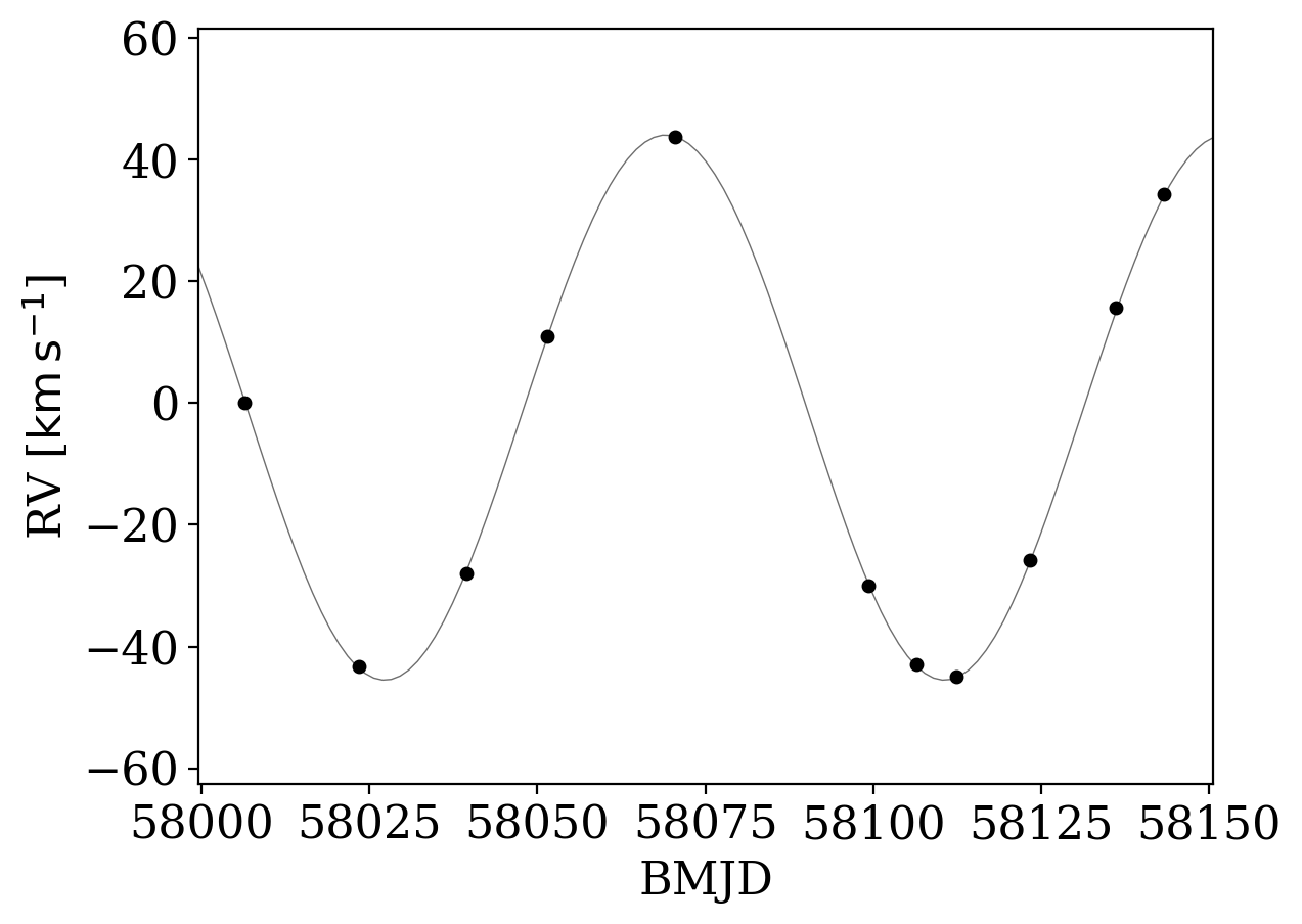
Let’s look at the values of the sample that was returned, and compare that to the values reported in Thompson et al. 2019, included below for convenience:
[13]:
samples.tbl["P", "e", "K"]
[13]:
| P | e | K |
|---|---|---|
| d | km / s | |
| float64 | float64 | float64 |
| 83.2977327639342 | 0.008612274267935767 | 44.76966704707342 |
Already these look very consistent with the values inferred in the paper!
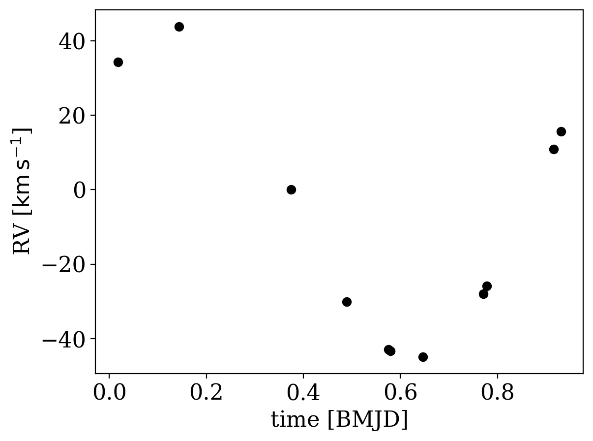
Let’s now also plot the data phase-folded on the period returned in the one sample we got from The Joker:
[14]:
_ = tres_data.plot(phase_fold=samples[0]["P"])
WARNING: AstropyDeprecationWarning: "phase_fold" was deprecated in version v1.3 and will be removed in a future version. Use argument "phase_fold_period" instead. [warnings]
At this point, since the data are very constraining, we could use this one Joker sample to initialize standard MCMC to generate posterior samplings in the orbital parameters for this system. We will do that below, but first let’s see how things look if we include both TRES and APOGEE data in our modeling.
Run The Joker with TRES+APOGEE data#
One of the challenges with incorporating data from the two surveys is that they were taken with two different spectrographs, and there could be instrumental offsets that manifest as shifts in the absolute radial velocities measured between the two instruments. The Joker now supports simultaneously sampling over additional parameters that represent instrumental or calibratrion offsets, so let’s take a look at how to run The Joker in this mode.
To start, we can pack the two datasets into a single list that contains data from both surveys:
[15]:
data = [apogee_data, tres_data]
Before we run anything, let’s try phase-folding both datasets on the period value we got from running on the TRES data alone:
[16]:
tres_data.plot(color=None, phase_fold_period=np.mean(samples["P"]))
apogee_data.plot(color=None, phase_fold_period=np.mean(samples["P"]))
[16]:
<Axes: xlabel='time [BMJD]', ylabel='RV [$\\mathrm{km\\,s^{-1}}$]'>
That looks pretty good, but the period is clearly slightly off and there seems to be a constant velocity offset between the two surveys, given that the APOGEE RV points don’t seem to lie in the RV curve. So, let’s now try running The Joker on the joined dataset!
To allow for an unknown constant velocity offset between TRES and APOGEE, we have to define a new parameter for this offset and specify a prior. We’ll put a Gaussian prior on this offset parameter (named dv0_1 below), with a mean of 0 and a standard deviation of 10 km/s, because it doesn’t look like the surveys have a huge offset.
[17]:
with pm.Model() as model:
    # The parameter that represents the constant velocity offset between
    # APOGEE and TRES:
    dv0_1 = xu.with_unit(pm.Normal("dv0_1", 0, 5.0), u.km / u.s)

    # The same extra uncertainty parameter as previously defined
    s = xu.with_unit(pm.Lognormal("s", -2, 1), u.km / u.s)

    # We can restrict the prior on prior now, using the above
    prior_joint = tj.JokerPrior.default(
        # P_min=16*u.day, P_max=128*u.day,
        P_min=75 * u.day,
        P_max=90 * u.day,
        sigma_K0=30 * u.km / u.s,
        P0=1 * u.year,
        sigma_v=25 * u.km / u.s,
        v0_offsets=[dv0_1],
        s=s,
    )

prior_samples_joint = prior_joint.sample(size=1_000_000, rng=rnd)
[18]:
# Run rejection sampling with The Joker:
joker_joint = tj.TheJoker(prior_joint, rng=rnd)
samples_joint = joker_joint.rejection_sample(
    data, prior_samples_joint, max_posterior_samples=256
)
samples_joint
[18]:
<JokerSamples [P, e, omega, M0, s, K, v0, dv0_1] (1 samples)>
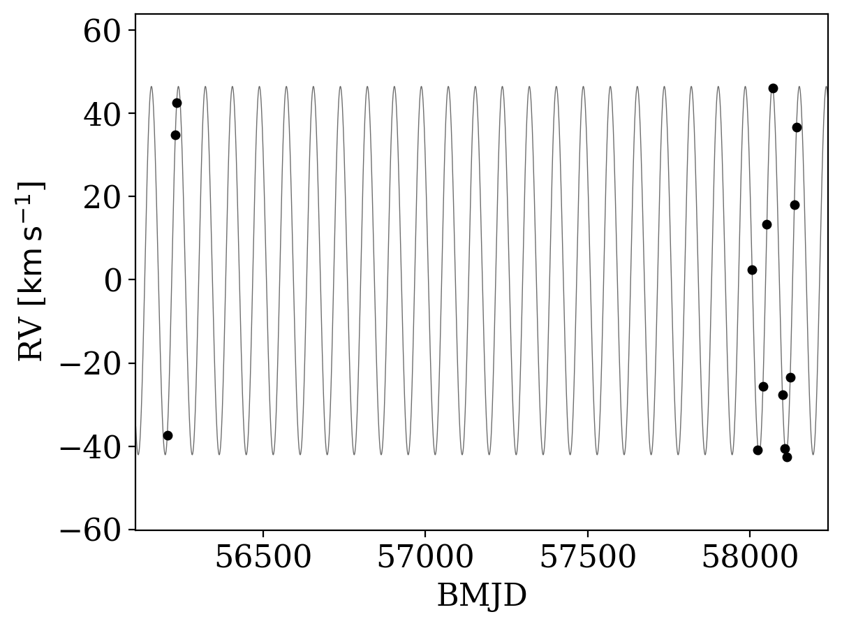
Here we again only get one sample back from The Joker, because these data are so constraining:
[19]:
_ = tj.plot_rv_curves(samples_joint, data=data)
Now, let’s fire up standard MCMC, using the one Joker sample to initialize. We will use the NUTS sampler in pymc3 to run here. When running MCMC to model radial velocities with Keplerian orbits, it is typically important to think about the parametrization. There are several angle parameters in the two-body problem (e.g., argument of pericenter, phase, inclination, etc.) that can be especially hard to sample over naïvely. Here, for running MCMC, we will instead sample over
\(M_0 - \omega, \omega\) instead of \(M_0, \omega\), and we will define these angles as pymc3_ext.distributions.Angle distributions, which internally transform and sample in \(\cos{x}, \sin{x}\) instead:
[20]:
from pymc_ext.distributions import angle

with pm.Model():
    # See note above: when running MCMC, we will sample in the parameters
    # (M0 - omega, omega) instead of (M0, omega)
    M0_m_omega = xu.with_unit(angle("M0_m_omega"), u.radian)
    omega = xu.with_unit(angle("omega"), u.radian)
    # M0 = xu.with_unit(angle('M0'), u.radian)
    M0 = xu.with_unit(pm.Deterministic("M0", M0_m_omega + omega), u.radian)

    # The same offset and extra uncertainty parameters as above:
    dv0_1 = xu.with_unit(pm.Normal("dv0_1", 0, 5.0), u.km / u.s)
    s = xu.with_unit(pm.Lognormal("s", -2, 0.5), u.km / u.s)

    prior_mcmc = tj.JokerPrior.default(
        P_min=16 * u.day,
        P_max=128 * u.day,
        sigma_K0=30 * u.km / u.s,
        P0=1 * u.year,
        sigma_v=25 * u.km / u.s,
        v0_offsets=[dv0_1],
        s=s,
        pars={"M0": M0, "omega": omega},
    )

    joker_mcmc = tj.TheJoker(prior_mcmc, rng=rnd)
    mcmc_init = joker_mcmc.setup_mcmc(data, samples_joint)

    trace = pm.sample(
        tune=1000, draws=500, start=mcmc_init, random_seed=seed, cores=1, chains=2
    )
Auto-assigning NUTS sampler...
Initializing NUTS using jitter+adapt_diag...
Sequential sampling (2 chains in 1 job)
NUTS: [__M0_m_omega_angle1, __M0_m_omega_angle2, __omega_angle1, __omega_angle2, dv0_1, s, e, P, K, v0]
/opt/hostedtoolcache/Python/3.11.9/x64/lib/python3.11/site-packages/rich/live.py:231: UserWarning: install
"ipywidgets" for Jupyter support
  warnings.warn('install "ipywidgets" for Jupyter support')
Sampling 2 chains for 1_000 tune and 500 draw iterations (2_000 + 1_000 draws total) took 92 seconds.
There were 31 divergences after tuning. Increase `target_accept` or reparameterize.
We recommend running at least 4 chains for robust computation of convergence diagnostics
The effective sample size per chain is smaller than 100 for some parameters.  A higher number is needed for reliable rhat and ess computation. See https://arxiv.org/abs/1903.08008 for details
We can now use pymc3 to look at some statistics of the MC chains to assess convergence:
[21]:
az.summary(trace, var_names=prior_mcmc.par_names)
[21]:
| mean | sd | hdi_3% | hdi_97% | mcse_mean | mcse_sd | ess_bulk | ess_tail | r_hat | |
|---|---|---|---|---|---|---|---|---|---|
| P | 83.161 | 0.014 | 83.136 | 83.190 | 0.001 | 0.001 | 304.0 | 363.0 | 1.01 |
| e | 0.003 | 0.002 | 0.000 | 0.007 | 0.000 | 0.000 | 149.0 | 177.0 | 1.01 |
| omega | 0.467 | 1.178 | -1.920 | 2.829 | 0.059 | 0.078 | 326.0 | 307.0 | 1.01 |
| M0 | -0.035 | 1.180 | -2.415 | 2.337 | 0.060 | 0.074 | 324.0 | 307.0 | 1.01 |
| s | 0.222 | 0.053 | 0.144 | 0.328 | 0.003 | 0.002 | 300.0 | 511.0 | 1.00 |
| K | -44.732 | 0.102 | -44.939 | -44.549 | 0.005 | 0.004 | 344.0 | 313.0 | 1.00 |
| v0 | 2.147 | 0.576 | 1.020 | 3.211 | 0.034 | 0.024 | 290.0 | 425.0 | 1.01 |
| dv0_1 | -2.596 | 0.593 | -3.748 | -1.481 | 0.035 | 0.024 | 292.0 | 372.0 | 1.01 |
We can then transform the MCMC samples back into a JokerSamples instance so we can manipulate and visualize the samples:
[22]:
mcmc_samples = tj.JokerSamples.from_inference_data(prior_joint, trace, data=data)
mcmc_samples = mcmc_samples.wrap_K()
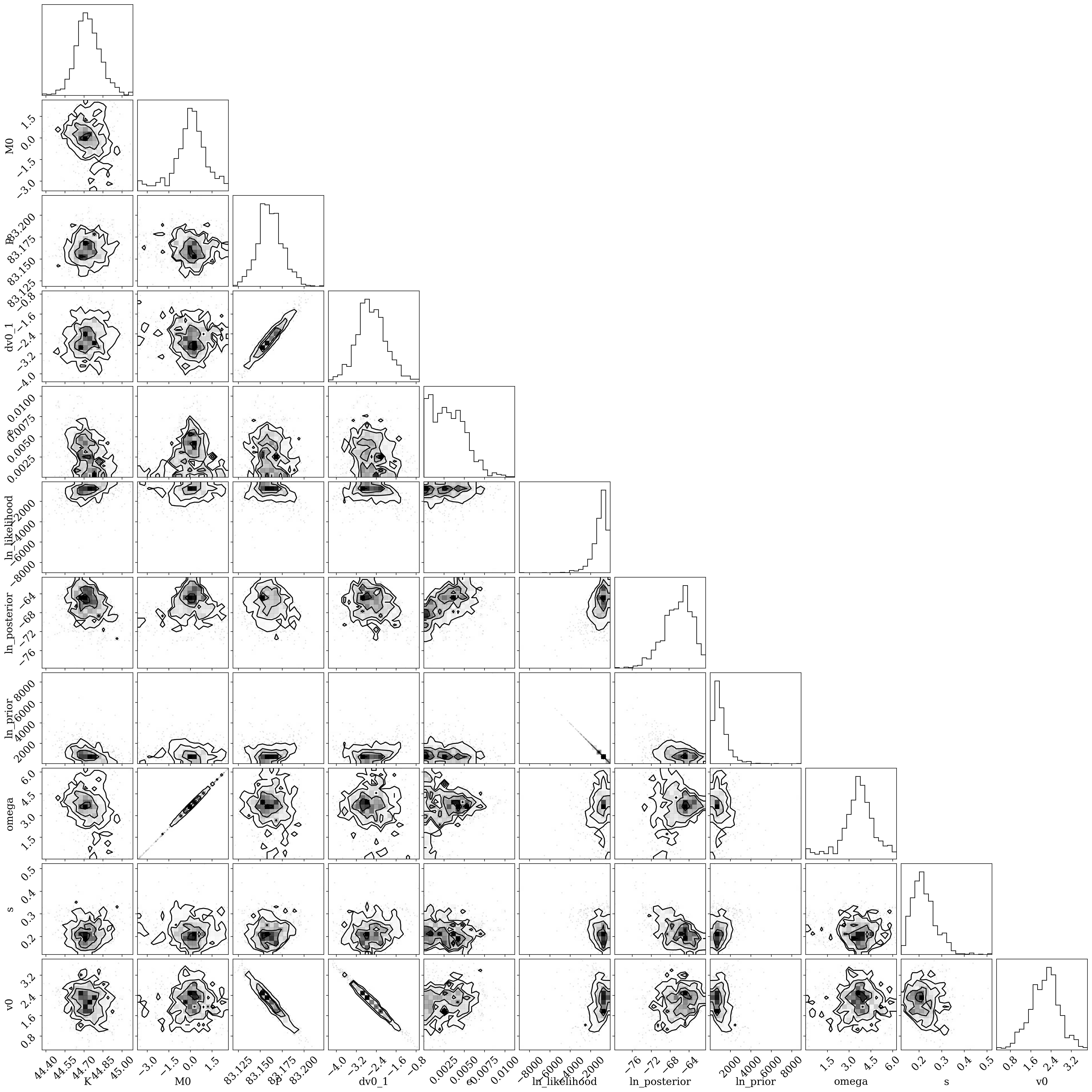
For example, we can make a corner plot of the orbital parameters (note the strong degenceracy between M0 and omega! But also note that we don’t sample in these parameters explicitly, so this shouldn’t affect convergence):
[23]:
df = mcmc_samples.tbl.to_pandas()
_ = corner.corner(df)
WARNING:root:Pandas support in corner is deprecated; use ArviZ directly
WARNING:root:Too few points to create valid contours
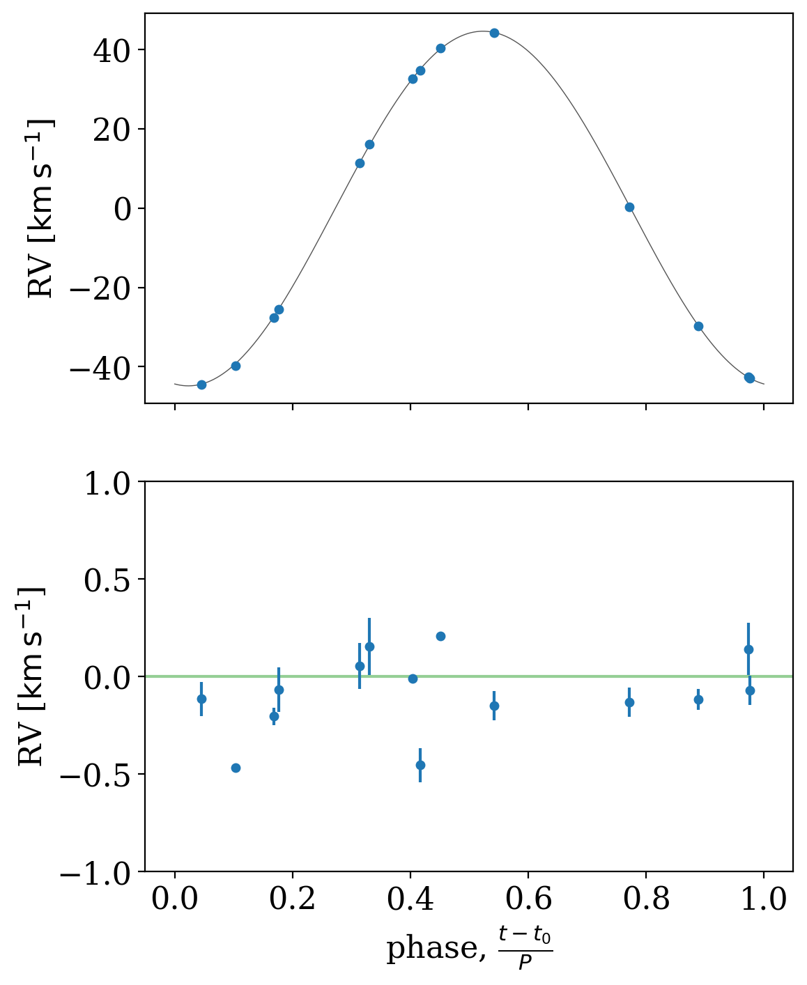
We can also use the median MCMC sample to fold the data and plot residuals relative to our inferred RV model:
[24]:
fig, axes = plt.subplots(2, 1, figsize=(6, 8), sharex=True)

_ = tj.plot_phase_fold(mcmc_samples.median_period(), data, ax=axes[0], add_labels=False)
_ = tj.plot_phase_fold(mcmc_samples.median_period(), data, ax=axes[1], residual=True)

for ax in axes:
    ax.set_ylabel(f"RV [{apogee_data.rv.unit:latex_inline}]")

axes[1].axhline(0, zorder=-10, color="tab:green", alpha=0.5)
axes[1].set_ylim(-1, 1)
[24]:
(-1.0, 1.0)
Finally, let’s convert our orbit samples into binary mass function, \(f(M)\), values to compare with one of the main conclusions of the Thompson et al. paper. We can do this by first converting the samples to KeplerOrbit objects, and then using the .m_f attribute to get the binary mass function values:
[25]:
mfs = u.Quantity(
    [mcmc_samples.get_orbit(i).m_f for i in rnd.choice(len(mcmc_samples), 1024)]
)
plt.hist(mfs.to_value(u.Msun), bins=32)
plt.xlabel(rf"$f(M)$ [{u.Msun:latex_inline}]")
# Values from Thompson et al., showing 1-sigma region
plt.axvline(0.766, zorder=100, color="tab:orange")
plt.axvspan(
    0.766 - 0.00637, 0.766 + 0.00637, zorder=10, color="tab:orange", alpha=0.4, lw=0
)
[25]:
<matplotlib.patches.Rectangle at 0x7fa37f438190>
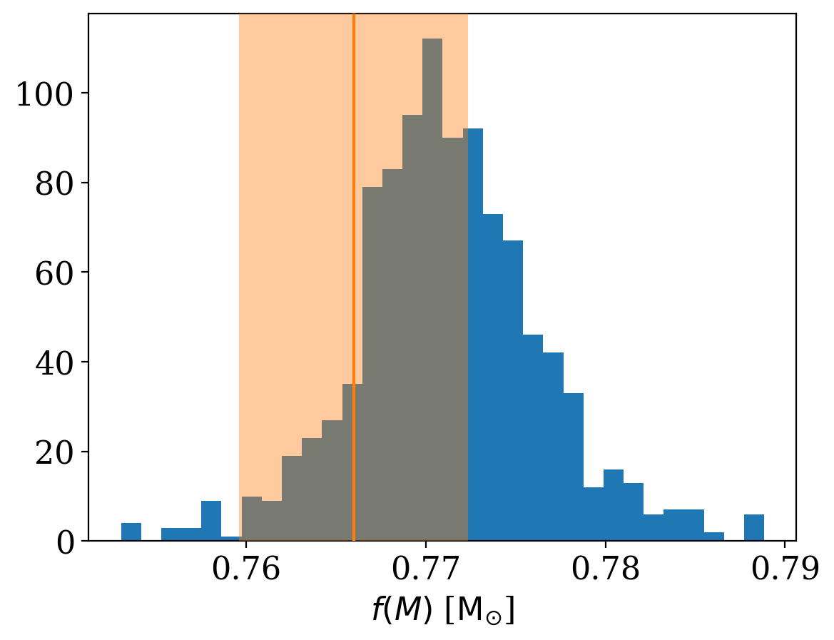
In the end, using both the APOGEE and TRES data, we confirm the results from the paper, and find that the binary mass function value suggests a large mass companion. A success for reproducible science!