
The Joker [YO-ker] /’joʊkər/#
Introduction#
The Joker [1] is a custom Monte Carlo sampler for the two-body problem that generates posterior samplings in Keplerian orbital parameters given radial velocity observations of stars. It is designed to deliver converged posterior samplings even when the radial velocity measurements are sparse or very noisy. It is therefore useful for constraining the orbital properties of binary star or star-planet systems. Though it fundamentally assumes that any system has two massive bodies (and only the primary is observed), The Joker can also be used for hierarchical systems in which the velocity perturbations from a third or other bodies are much longer than the dominant companion. See the paper [2] for more details about the method and applications.
Note
New with v1.3, thejoker is no longer based on pymc3 and is now instead built
on pymc. If you used thejoker previously
with pymc3, you will have to upgrade and modify some code to use the new version
of pymc instead.
Getting started#
Generating samples with The Joker requires three things:
The data,
thejoker.RVData: radial velocity measurements, uncertainties, and observation timesThe priors,
thejoker.JokerPrior: the prior distributions over the parameters in The JokerThe sampler,
thejoker.TheJoker: the work horse that runs the rejection sampler
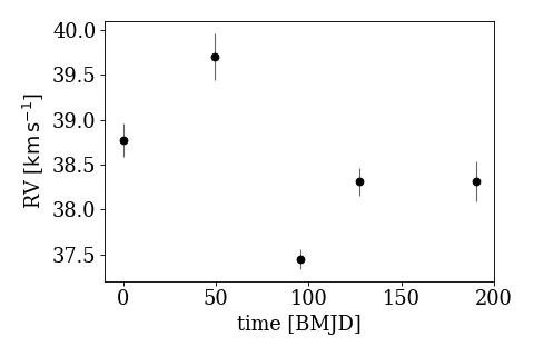
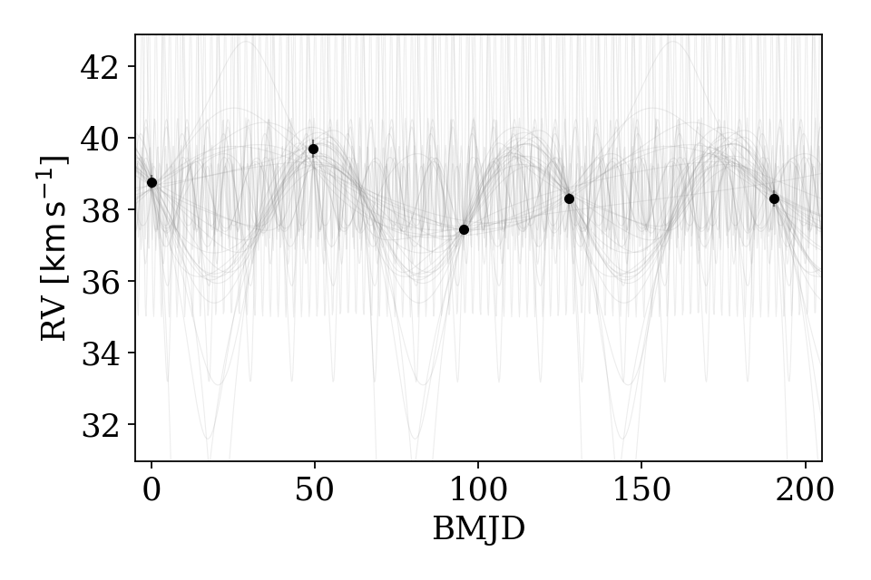
Here, we’ll work through a simple example to generate posterior samples for orbital parameters given some sparse, simulated radial velocity data (shown below). We’ll first use these plain arrays to construct a ~thejoker.RVData object:
>>> import astropy.units as u
>>> import thejoker as tj
>>> t = [0., 49.452, 95.393, 127.587, 190.408]
>>> rv = [38.77, 39.70, 37.45, 38.31, 38.31] * u.km/u.s
>>> err = [0.184, 0.261, 0.112, 0.155, 0.223] * u.km/u.s
>>> data = tj.RVData(t=t, rv=rv, rv_err=err)
>>> ax = data.plot()
>>> ax.set_xlim(-10, 200)
(Source code, 2.0x.png, png, hires.png, pdf)
We next need to specify the prior distributions for the parameters of The Joker. The
default prior, explained in the docstring of thejoker.JokerPrior.default(),
assumes some reasonable defaults where possible, but requires specifying the minimum and
maximum period to sample over, along with parameters that specify the prior over the
linear parameters in The Joker (the velocity semi-amplitude, K, and the systemic
velocity, v0):
>>> import numpy as np
>>> prior = tj.JokerPrior.default(
...     P_min=2*u.day, P_max=256*u.day,
...     sigma_K0=30*u.km/u.s,
...     sigma_v=100*u.km/u.s
... )
With the data and prior created, we can now instantiate the sampler object and run the rejection sampler:
>>> joker = tj.TheJoker(prior)
>>> prior_samples = prior.sample(size=100_000)
>>> samples = joker.rejection_sample(data, prior_samples)
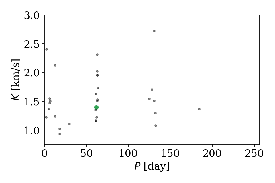
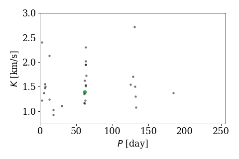
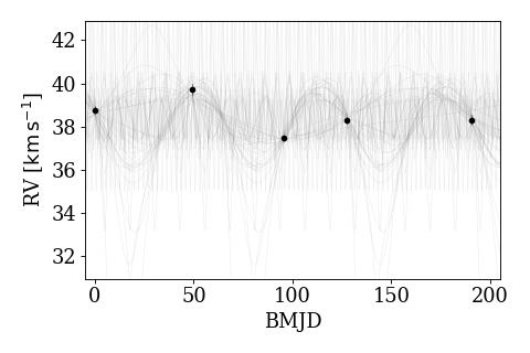
Of the 100,000 prior samples we generated, only a handful pass the rejection sampling step of The Joker. Let’s visualize the surviving samples in the subspace of the period \(P\) and velocity semi-amplitude \(K\). We’ll also plot the true values as a green marker. As a separate plot, we’ll also visualize orbits computed from these posterior samples (check the source code below to see how these were made):

(2.0x.png, png, hires.png, pdf)
(2.0x.png, png, hires.png, pdf)
Footnotes